Grand Canonical Generators

GCG samples the μVT ensemble: a distribution over particle number N and geometry X, given the chemical potential μ.

Why open systems are hard

Many systems involve particles entering and leaving the system. Examples include carbon capture in porous materials and hydration of protein pockets.

These open systems are described by the grand canonical (μVT) ensemble, a distribution over the particle number N and the coordinates X:

\[ \pi(N,X\mid\beta,\mu,c)=\frac{\gamma_\mu(N,X;c)}{\Xi},\qquad \gamma_\mu(N,X;c)=\frac{e^{-\beta U_N(X;c)+\beta\mu N}}{N!\,\Lambda^{3N}}, \]

Ξ is the intractable grand canonical partition function, U_N is the potential energy, and c is the context (for example, the porous material).

GCMC is slow

Insertion and deletion moves often overlap existing particles. Acceptance is low and correlation times are long.

Boltzmann generators fix N

They can draw independent samples rapidly, but only for a fixed N (the canonical ensemble).

\[ \pi(X\mid N)=\frac{e^{-\beta U_N(X)}}{Z_N} \]

Two designs

We train on GCMC data at a few chemical potentials, then generate configurations at new ones.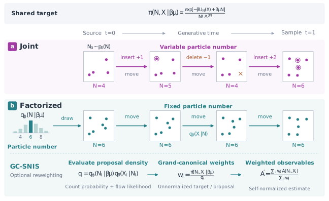

1. Joint GCG

One variable-size generative process models (N, X) together and is conditioned on μ.

\[ q_\theta(N,X\mid\mu) \]

It is variable-size, but must learn the μ dependence from data. It has no tractable likelihood.

2. Factorized GCG

A particle-number model feeds a conditional Boltzmann generator.

\[ q(N,X\mid\mu)=q_\phi(N\mid\mu)\;q_\theta(X\mid N) \]

It is variable-size, encodes the μ dependence analytically, and has a tractable likelihood.

Why the factorization helps

The grand canonical distribution splits into a particle-number part and a canonical part:

\[ \pi(N,X\mid\mu)=\underbrace{\pi(N\mid\mu)}_{\propto\, e^{\beta\mu N} Z_N/(N!\,\Lambda^{3N})}\;\underbrace{\pi(X\mid N)}_{\text{canonical, independent of }\mu} \]

Any Boltzmann generator. The configuration part q_θ(X | N) can use any architecture that conditions on N.
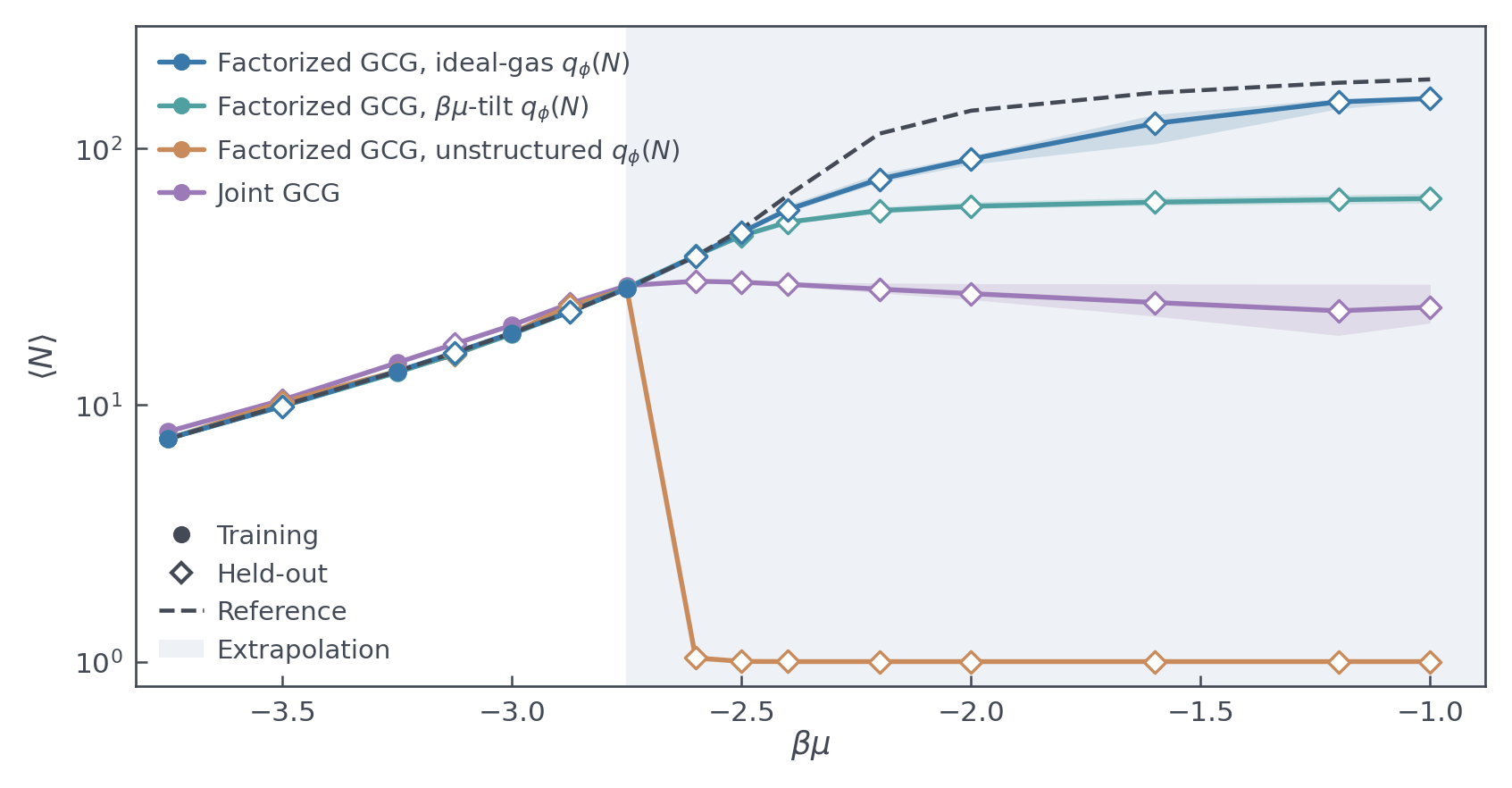
Known dependence is analytic. We hard-code the tilt and the factorial. The network learns only the residual, which holds the ratios of canonical partition functions Z_N: \[ \log q_\phi(N\mid\mu)=\beta\mu N-\log N!+r_\phi(N)-\log C(\mu) \] Because r_φ does not depend on μ, the model transfers to unseen chemical potentials.
Tractable joint likelihood. The product q_φ(N | μ) q_θ(X | N) is a normalized density. It supports self-normalized importance sampling (SNIS) for inference-time correction.

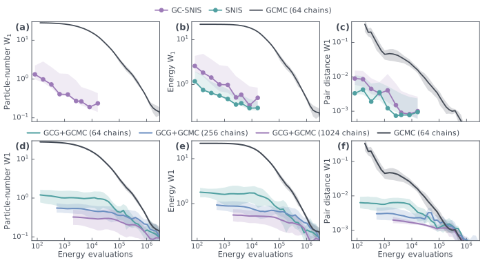
Samples from either design can also start GCMC chains. This needs no likelihood.

Results

Lennard-Jones fluid

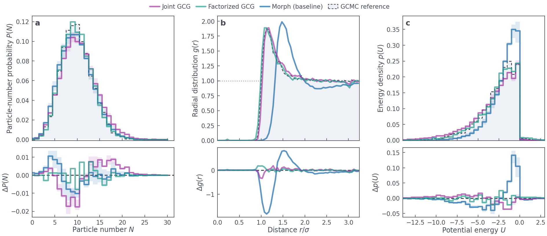
Both GCG variants learn the correct radial distribution function and the energy distribution. Naively using an existing variable size model made for molecular design instead of sampling, Morph, overestimates the energy.

Generalization across chemical potentials

Using the Factorized GCG, we can hard-code known terms analytically and improve transfer to unseen chemical potentials.

Particle-number transfer to unseen chemical potentials.

Inference-time correction

The joint likelihood gives self-normalized importance weights for each generated state:

\[ w(N,X)=\frac{\gamma_\mu(N,X;c)}{q_\phi(N\mid\mu)\,q_\theta(X\mid N)},\qquad \langle O\rangle\approx\frac{\sum_i w_i\,O(N_i,X_i)}{\sum_i w_i} \]

Stratification. To reduce variance, we draw a fixed number of configurations for each particle number N, instead of sampling N at random. This keeps coverage across all relevant particle numbers.

Conditional SNIS reweights the configurations at each fixed N. It uses the canonical weights below. It keeps the learned q_φ(N | μ). \[ w(X\mid N)=\frac{e^{-\beta U_N(X;c)}}{q_\theta(X\mid N)} \]
GC-SNIS also corrects the particle-number probabilities. It uses the full weights w(N, X) above.

Inference-time correction of Factorized GCG on LJ with SNIS and GCMC. — Inference-time correction of Factorized GCG on LJ with SNIS (top) and GCMC (bottom).

Methane adsorption in MFI zeolite

In a realistic application, Factorized GCG learns the correct distribution of methane molecules in the zeolite.

GCMC moves in small steps, so its samples stay correlated. GCG generates independent configurations.

Future work

Make GCG transferable across systems, to amortize the cost of data collection.
Use energy-based training to reduce the need for training data. These methods are also called diffusion samplers or neural samplers.
Use likelihood flow maps for fast SNIS.
Try autoregressive models. They have variable size and tractable likelihoods.

Citation

@article{burger2026grand,
  title   = {Grand Canonical Generators},
  author  = {Burger, Andreas and Franke, Malte and Mucko, Luka and Jorner, Kjell and Aspuru-Guzik, Alan},
  journal = {arXiv preprint arXiv:2610.00683},
  year    = {2026},
  url     = {https://arxiv.org/abs/2610.00683}
}